.svg)
Industry insights
Jun 16, 2023
Time series analysis: a gentle introduction
Explore the fundamentals of time series analysis in this comprehensive article. Learn about key concepts, use cases, and types of time series analysis, and discover models, techniques, and methods to analyze time series data.


Introduction
The proliferation of technologies like IoT and mobile devices, the internet, data transmission methods, and cloud computing means we live in a data-centric world. And the ability to collect, analyze and derive meaningful insights from data is a crucial driver of success for organizations across nearly every sector.
There are many types of data that can be collected for analysis purposes. Among them, time series data. In a nutshell, time series data is a collection of observations or measurements recorded sequentially, typically at regular, consistent intervals (e.g., every second, every minute, hourly, daily, weekly, or monthly). Common examples of time series data include stock prices and measurements from telemetry devices (e.g., temperature or pressure sensors).
Time series data involves different types of variables that change over time. For example, altitude, latitude, longitude, and speed are four variables that define the location and velocity of a plane in the sky.
What is time series analysis?
Time series analysis refers to all the methods, techniques, and models you can use to monitor and extract insights from time series data and its evolution in time. For instance, if we were to analyze time series data collected from the plane we mentioned earlier, we would be able to answer questions like:
- What is the aircraft's current location and how long will it take to reach its destination?
- How well is the plane maintaining its speed and cruising altitude?
- Are there any sudden altitude drops or speed changes that could indicate potential safety concerns or turbulence?
- Are there any recurring patterns in flight data that suggest maintenance is required?
- Was the flight path the most efficient, or are there opportunities to save fuel and time in the future?
Why is time series analysis needed?
Companies and individuals rely on time series analysis to extract meaningful and actionable insights from data. Here’s a list of different ways time series analysis can be leveraged:
- Forecasting. By analyzing time series data, organizations are empowered to predict the likelihood of future events and outcomes.
- Detecting trends and patterns. Analyzing time series data helps businesses identify patterns and trends, and understand their underlying causes.
- Understanding data relationships. Time series analysis enables organizations to understand the relationship between different data variables, and how they influence each other over time.
- Anomaly detection. Time series analysis is frequently used to identify unusual occurrences or anomalies.
- Risk management. Time series analysis can help in risk assessment and management by modeling and predicting adverse events or volatilities.
- Decision making. Many decision-making processes rely on understanding how a data variable changes over time. In such scenarios, time series analysis can inform and guide decisions.
Improving operational efficiency. Businesses can use time series analysis to gain real-time visibility into their operations. This way, they can allocate resources efficiently, minimize costs, and quickly react to changing conditions.
What is time series analysis used for?
Time series analysis has broad applications across different industries and disciplines. Depending on the use case, analysis can be performed on historical data, or in real time.
Analyzing historical data
Analyzing historical time series data is a good option in scenarios where you aim to identify long-term trends and patterns, and there’s no pressure or business need to extract insights instantly, as soon as data is collected. Instead, data can be analyzed at a later date. Examples include:
- Analyzing economic indicators to forecast economic growth or recession.
- Analyzing sales data from the past year to predict future sales trends.
- Analyzing past weather data to predict weather patterns and perform climate change studies.
- Analyzing energy usage from the last six months to identify patterns and improve efficiency.
- Analyzing website traffic data weekly to determine traffic patterns and predict conversion rates.
- Analyzing health data to predict the spread of diseases.
Real-time use cases
There are scenarios with a limited window of opportunity to extract insights from time series data and act on them. In such cases, data needs to be analyzed in real time, as soon as it becomes available. For instance:

Time series car data collected and visualized in real time using a waveform graph. Source.
Time series analysis: key concepts
We will now discuss some key concepts data enthusiasts need to be aware of if they plan to analyze time series data.
Time series vs. pooled vs. cross-sectional data
Time series data is one of the most frequent data structures used in statistical analysis. But how does it compare to other common types of data, specifically cross-sectional and pooled data? And how can you combine them to draw meaningful statistics and insights?
As previously mentioned, time series data consists of observations about how one or more variables evolve in time. For instance, a retail organization may collect sales figures at the end of every month to analyze the monthly sales of different product categories in its stores. The sales figures compiled over time form a time series data set.
On the other hand, cross-sectional data is like a snapshot that gives a glimpse of a particular situation or state at a specific point in time. For example, the retail business could collect cross-sectional data on the number and size of stores in various cities to analyze the distribution and growth of its presence across different regions.
Finally, pooled data is a combination of information from different sources into a single dataset. Pooled data often comprises time series information, as well as cross-sectional data. The retail organization might pool time series data on monthly sales revenue for multiple retail stores and cross-sectional data on store attributes (size, location, number of employees) to analyze sales trends and explore relationships between store characteristics and sales performance.
Time series components
There are several components that data scientists and analysts need to take into account when analyzing time series data:
- Trend refers to the overall evolution of data over a long period of time. Trends can be upward (increasing), downward (decreasing), or null (no clear or significant movement in the data series over time). Trend analysis is crucial for detecting long-term patterns and identifying potential opportunities or risks.
- Seasonality refers to periodic data variations that occur at regular time intervals. For example, suppose you're analyzing shopping habits over a calendar year. There’s a good chance you’ll see sales spike during holidays like Christmas and drop to lower levels for the rest of the year. Analyzing seasonality is essential to understanding repeatable patterns and improving forecasting accuracy.
- Cyclicity implies data fluctuations that occur over a very long time period (years or even decades). Consider, for instance, a dataset of annual population growth for a country over several decades. Upon analyzing the data, you may observe a cyclic pattern where the population growth rate experiences periods of acceleration (e.g., during periods of economic prosperity), followed by periods of deceleration (e.g., during economic downturns). Cyclicity analysis enables us to uncover hidden patterns, identify recurring trends, improve forecasting, and enhance decision-making.
- Randomness or irregularity implies unexpected, unpredictable, or uncommon events and scenarios that impact data somehow. Let's consider a daily stock price dataset. Stock prices are typically recorded at the end of each trading day. However, there may be instances where no trading activity occurred due to public holidays or market closures. As a result, there will be gaps or irregularities in the time series data, with missing data points on certain days. Failing to handle these irregularities (e.g., through techniques like data imputation and mean substitution) can lead to biased analysis results or inaccurate interpretations.

Learn more about:
Stationarity
In time series analysis, data can be classified as stationary and non-stationary. Here's how they are different:
- Stationary. Data remains relatively constant, with consistent statistical properties and relationships between data points.
- Non-stationary. Data and statistical properties change over time, indicating trends, seasonality, or patterns.

Stationary vs. non-stationary time series data. Source.
Most raw time series data, like stock prices, temperature, or electricity usage, is non-stationary because its stats change over time. Yet, many statistical models and prediction techniques work better with stationary data. That's because it's easier to model and predict something that stays consistent over time.
So, before analyzing time series data, you need to check if your data is stationary. You can do this using tests like Augmented Dickey-Fuller (ADF), Kwiatkowski-Phillips-Schmidt-Shin (KPSS), and Phillips-Perron (PP).
If your data turns out to be non-stationary, you can transform it to be stationary. This can be done in several ways, such as differencing, applying a logarithmic transformation, removing trends, or adjusting for seasonal changes.
Learn more about stationarity in time series analysis
Autocorrelation
Autocorrelation is about understanding how a current data point is influenced by all past data points. It's basically comparing the same information at different points in time. For instance, when studying daily temperatures, autocorrelation tells us how today's temperature relates to those of previous days. If there's a high autocorrelation, today's temperature will likely be similar to yesterday's, while a low auto correlation suggests otherwise.
Meanwhile, partial autocorrelation focuses on the relationship between a current data point and a specific past data point, ignoring any other data points in between. It's like asking, "How much is today's weather influenced by the weather exactly two days ago, ignoring the influence of yesterday's weather?"

Autocorrelation and partial autocorrelation. Source.
Looking at autocorrelation and partial autocorrelation helps us spot patterns and trends over time in our data. This is useful when we're trying to make predictions about the future, like forecasting the weather or predicting stock market trends.
Learn how to calculate and plot autocorrelation and partial autocorrelation with Python
Types of time series analysis
There are numerous types of time series analysis. We cover the most common ones below; as you will see, each type of analysis has different characteristics and serves different purposes.
Time series analysis models, techniques, and methods
There’s an abundance of statistical, mathematical, and machine learning techniques, methods, and models data professionals can use to analyze and extract value from time series data. Here’s a list of the most popular, commonly-used ones:
Autoregression
Autoregression is a way of predicting future data values based on past ones, by using regression equations. Think of it like forecasting tomorrow's weather using temperatures from previous days. This technique, which assumes a direct relationship between past and future values, is often applied in finance to estimate future stock prices.
Learn how to implement an autoregressive model for time series with Python
Moving average
The moving average technique smooths out short-term data fluctuations and highlights trends or cycles. Moving averages can be used on different windows of time. For example, if you’re analyzing website traffic, you could apply a moving average to a seven-day time period to identify trends. On the other hand, a utility company analyzing power usage might use a 24-hour moving average to smooth out hourly fluctuations and better understand the pattern of electricity consumption.
There are several different types of moving averages, including:
- Simple moving average (SMA). Treats every data point equally. Suitable for analyzing longer time frames or scenarios where data doesn’t change rapidly (e.g., tracking average annual rainfall in a city).
- Weighted moving average (WMA). Gives more importance to the most recent data points. Helpful when dealing with medium-term time frames or when data shows moderate fluctuations (for example, analyzing the most recent customer feedback).
- Exponential moving average (EMA). Also a weighted average, but it assigns significantly more weight to the latest data points. It’s the best choice if you're dealing with data that shifts rapidly and you need to respond quickly to these changes (for instance, you’re monitoring real-time fluctuations in cryptocurrency values).

An example of using the moving average technique on stock market data. Source.
Learn how to calculate moving averages
ARMA
ARMA, short for Autoregressive Moving Average, is a forecasting model that blends two mechanisms: autoregression and moving averages.
The autoregressive part indicates that the analysis output relies on prior data values. Think of this as today's weather depending on the past few days' weather. The moving average component, on the other hand, accounts for shifts in the data that the autoregressive part can't explain by itself. For example, a sudden heavy rainfall could drastically drop the temperature in a short period, which is something that would not be directly connected to the temperatures of the previous days.
ARMA is most useful when dealing with stationary time series data that shows no obvious trends or seasonal patterns. A practical use could be for a company making machine parts. They could use ARMA to predict how much raw material they'll need each week, assuming their needs don't have clear patterns or seasonal changes.
Learn more about the ARMA model
ARIMA and SARIMA
ARIMA, which stands for Autoregressive Integrated Moving Average, and SARIMA, or Seasonal Autoregressive Integrated Moving Average, are commonly used forecasting models. They're frequently implemented using the Box-Jenkins approach.
ARIMA is like an upgraded version of ARMA, and it's used for studying datasets that show trends. ARIMA combines elements of ARMA and differencing techniques to eliminate trends from time series, thus making data easier to analyze.
SARIMA takes things one step further. This model is used to analyze time series data showing a repeating pattern at certain times, like higher ice cream sales during summer — this is what we call seasonal variation.
One important thing to remember is that both ARIMA and SARIMA focus solely on one data variable, like temperature readings over time. They predict future values based on past trends in that data, without considering the influence of other factors.
Learn more about time series forecasting with ARIMA and SARIMA
Box-Jenkins multivariate models
The Box-Jenkins approach is often linked with single-variable forecasting models like ARIMA and SARIMA. But it can also be used with multi-variable (multivariate) models like VAR and VARMA. These latter models are great when you need to look at several variables that impact each other. For example, when you want to predict things like a country's GDP, inflation, and job rates - all of which affect one another - these models come in handy.
Learn more about multivariate time series analysis
Exponential smoothing
Exponential smoothing is a popular method in time series analysis. Like the exponential moving average, it calculates the average from past data points, with less importance given to older data. But while the exponential moving average is used to identify trends, the purpose of exponential smoothing is to predict future outcomes.
There are different types of exponential smoothing:
- Simple exponential smoothing - used for analyzing data without any noticeable trends or seasonal changes. For example, an internet service provider could use this method to forecast daily network usage in a data center.
- Double exponential smoothing (also known as Holt's linear exponential smoothing) - used for analyzing data with a clear trend over time. An example use case could be predicting the increasing number of app downloads for a popular mobile game.
- Triple exponential smoothing (or Holt-Winters exponential smoothing) - useful when data has both a trend and a seasonal pattern. For example, you can use this method to forecast hotel bookings in a tourist location, which typically rise during certain seasons (like summer) and increase yearly as the hotel becomes more well-known.

Learn more about exponential smoothing and time series analysis
Machine learning
Machine learning (ML) models and methods are becoming increasingly important for time series analysis, especially when dealing with large datasets. Technologies like RNN (recurrent neural network) and LSTM (long short-term memory networks) can capture complex patterns and dependencies in time series data. Plus, they can learn from historical values and make accurate predictions.
A key aspect of machine learning models in time series analysis is their applicability in real-time scenarios. ML models can integrate with streaming data sources, analyze large volumes of data, and generate real-time predictions or classifications. This is crucial for applications that require immediate responses, such as anomaly detection or real-time monitoring systems.
Learn about ML approaches for time series analysis
Python libraries for time series analysis
Due to its simplicity, readability, flexibility, and scalability, Python is the language of choice for many data professionals. A rich and diverse ecosystem of Python libraries is available to data scientists looking to analyze time series data. We list the most popular ones in the following table (note that they are all open source and free to use):
Challenges of time series analysis
While time series data has plenty of applications and brings plenty of benefits, analyzing it is a complex affair. What type(s) of analysis should you perform? What’s the best analysis model for your use case? How do you handle irregularities? How can you make data non-stationary? How do you account for seasonality? These are a few of the many questions and challenges you’ll have to address along the way.
But analyzing time series data is just the last step of a much bigger process. Before there’s anything to analyze, you first need to collect raw data, transform and process it, and store it somewhere. The emergence of data streaming and stream processing technologies in the past decade has revolutionized the field of time series analysis and data mining. These types of technologies allow us to collect, process, and analyze time series data as soon as it’s generated. This way, data can be used not only for historical analysis, but also to power real-time use cases like fraud detection and predictive maintenance in manufacturing.
However, building and managing a data pipeline that’s able to ingest, process, store, and analyze time series data in real time means more moving pieces, additional complexity, and extra headaches. See, for example, how hard it is to scale stream processing infrastructure to deal with vast volumes of data. Or learn about the challenges of handling streaming time series data.
The final point relates to machine learning. ML models are becoming increasingly used in time series analysis (especially for real-time use cases) — they’re significantly more efficient than manual analysis, and they’re well suited for handling vast amounts of high-frequency time series data. The tradeoff? There are numerous challenges involved in getting an ML model from prototype to production. Among them:
- It’s difficult and time-consuming to transform time series data into a suitable format for analysis.
- There are plenty of tough choices to make. For example, should you choose an ML algorithm that’s easier to scale, or one that’s harder to scale, but more accurate?
- Testing and deploying ML models can be a nightmare, especially for data scientists unfamiliar with software development best practices and engineering monitoring tools.
There are significant knowledge and skill differences between data engineers and data scientists, the two main roles involved in ML time series analysis. This gap adds additional complexity and needs to be bridged somehow.
Conclusion
As we have seen, analyzing time series data is vital for numerous industries: finance and banking, meteorology, healthcare, manufacturing, software development, transportation, and many, many more. Time series data analytics enable organizations across the board to monitor and optimize their operations, discover trends and patterns, predict future outcomes, make data-driven decisions, and instantly react to changing conditions.
On the flip side, collecting, processing, and analyzing time series data to gain actionable insights can be a daunting undertaking. If you’re looking for a way to simplify the process of extracting value from time series data, consider giving Quix a try. Founded by Formula 1 engineers with intimate knowledge of high-velocity time series data, Quix is a Python stream processing platform.
With Quix, data scientists are empowered to collect time series data from various sources and process it in real time. Then they can build ML models to analyze data, test them with Git & CI/CD, and seamlessly deploy them to production — all of this with minimum involvement from ML and data engineers.
To learn more about Quix and how we can help you build ML pipelines for time series data in days rather than months, check out our documentation and get started with a free account.
Last updated:
Dec 12, 2023

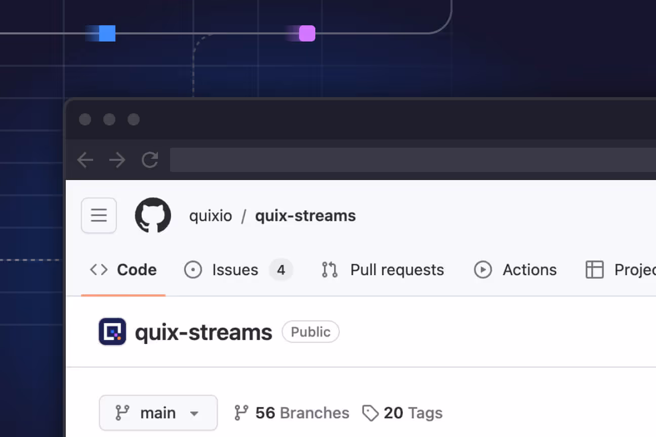
Check out the repo
Our Python client library is open source, and brings DataFrames and the Python ecosystem to stream processing.
Interested in Quix Cloud?
Take a look around and explore the features of our platform.
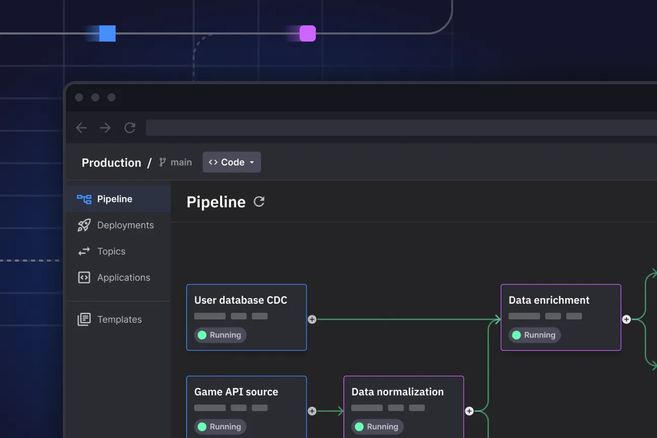
Interested in Quix Cloud?
Take a look around and explore the features of our platform.